Train a neural network
Once a neural network is created, it can be trained. To train a neural network, training data is required. If you have a system, that produces the output \(\underline{y}\), when given the input \(\underline{p}\) (see figure 6), \((\underline{p},\underline{y})\) represents one sample of training data.
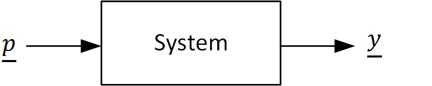
Figure 6: A system with input \(\underline{p}\) and output \(\underline{y}\)
For training neural networks usually more than one data sample is required to obtain good results. Therefore the training data is defined by an input matrix \(\widetilde{P}\) and an output (or target) matrix \(\widetilde{Y}\) containing \(Q\) samples of training data. For static systems (feed forward neural networks) it is only important that element \(q\) of the input matrix corresponds to element \(q\) of the output matrix (in any given order). For dynamic systems (recurrent neural networks) the samples have to be in the correct time order. For both systems, the training data should represent the system as good as possible.
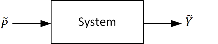
Figure 7: Generated training data set \(\widetilde{P}\) and \(\widetilde{Y}\) of a system
With the training data, the neural network can be trained. Training a neural network means, that all weights in the weight vector \(\underline{w}\), which contains all connection weights \(\widetilde{IW}\) and \(\widetilde{LW}\) and all bias weights \(\underline{b}\), are updated step by step, such that the neural network output \(\hat{\widetilde{Y}}\) matches the training data output (target) \(\widetilde{Y}\). The objective of this optimization is to minimize the error \(E\) (cost function) between neural network and system outputs.
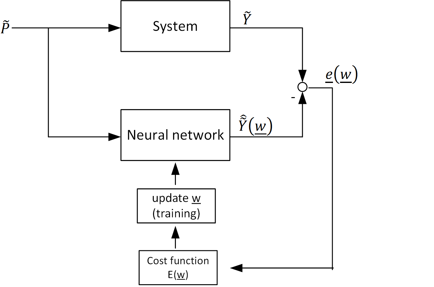
Figure 8: Training a neural network
Note
Generally there are different methods to calculate the error \(E\) (cost function) for neural network training. In pyrenn always the mean squared error is used, which is necessary to apply the Levenberg-Marquardt algorithm.
The training repeats adapting the weights of the weight vector \(\underline{w}\) until one of the two termination conditions becomes active:
- the maximal number of iterations (epochs) \(k_{max}\) is reached
- the Error is minimized to the goal \(E \leq E_{stop}\)
train_LM(): train with Levenberg-Marquardt Algorithm
The function train_LM() is an implementation of the Levenberg–Marquardt algorithm (LM) based on:
Levenberg, K.: A Method for the Solution of Certain Problems in Least Squares. Quarterly of Applied Mathematics, 2:164-168, 1944.
and
Marquardt, D.: An Algorithm for Least-Squares Estimation of Nonlinear Parameters. SIAM Journal, 11:431-441, 1963.
The LM algorithm is a second order optimization method that uses the Jacobian matrix \(\widetilde{J}\) to approximate the Hessian matrix \(\widetilde{H}\). In pyrenn the Jacobian matrix is calculated using the Real-Time Recurrent Learning (RTRL) algorithm based on:
Williams, Ronald J.; Zipser, David: A Learning Algorithm for Continually Running Fully Recurrent Neural Networks. In: Neural Computation, Nummer 2, Vol. 1 (1989), S. 270-280
Python
-
pyrenn.train_LM(P, Y, net[, k_max=100, E_stop=1e-10, dampfac=3.0, dampconst=10.0, verbose = False])¶ Trains the given neural network
netwith the training data inputsPand outputs (targets)Yusing the Levenberg–Marquardt algorithm.Parameters: - P (numpy.array) – Training input data set \(\widetilde{P}\), 2d-array of shape \((R,Q)\) with \(R\) rows (=number of inputs) and \(Q\) columns (=number of training samples)
- Y (numpy.array) – Training output (target) data set \(\widetilde{Y}\), 2d-array of shape \((S^M,Q)\) with \(S^M\) rows (=number of outputs) and \(Q\) columns (=number of training samples)
- net (dict) – a pyrenn neural network object created by
pyrenn.CreateNN() - k_max (int) – maximum number of training iterations (epochs)
- E_stop (float) – termination error (error goal), training stops when the \(E \leq E_{stop}\)
- dampfac (float) – damping factor of the LM algorithm
- dampconst (float) – constant to adapt damping factor of LM
- verbose (bool) – activates console outputs during training if True
Returns: a trained pyrenn neural network object
Return type:
Matlab
-
train_LM(P, Y, net, [k_max=100, E_stop=1e-10])¶ Trains the given neural network
netwith the training data inputsPand outputs (targets)Yusing the Levenberg–Marquardt algorithm.Parameters: - P (array) – Training input data set \(\widetilde{P}\), 2d-array with size \((R,Q)\) with \(R\) rows (=number of inputs) and \(Q\) columns (=number of training samples)
- Y (array) – Training output (target) data set \(\widetilde{Y}\), 2d-array with size \((S^M,Q)\) with \(S^M\) rows (=number of outputs) and \(Q\) columns (=number of training samples)
- net (struct) – a pyrenn neural network object created by
CreateNN() - k_max (int) – maximum number of training iterations (epochs)
- E_stop (double) – termination error (error goal), training stops when the \(E \leq E_{stop}\)
Returns: a trained pyrenn neural network object
Return type: struct
train_BFGS(): train with Broyden–Fletcher–Goldfarb–Shanno Algorithm (Matlab only)
The function train_BFGS() is an implementation of the Broyden–Fletcher–Goldfarb–Shanno algorithm (BFGS). The BFGS algorithm is a second order optimization method that uses rank-one updates specified by evaluations of the gradient \(\underline{g}\) to approximate the Hessian matrix \(H\). In pyrenn the gradient \(\underline{g}\) for BFGS is calculated using the Backpropagation Through Time (BPTT) algorithm based on:
Werbos, Paul: Backpropagation through time: what it does and how to do it. In: Proceedings of the IEEE, Nummer 10, Vol. 78 (1990), S. 1550-1560.
Matlab
-
train_BFGS(P, Y, net, [k_max=100, E_stop=1e-10])¶ Trains the given neural network
netwith the training data inputsPand outputs (targets)Yusing the Broyden–Fletcher–Goldfarb–Shanno algorithm.Parameters: - P (array) – Training input data set \(\widetilde{P}\), 2d-array with size \((R,Q)\) with \(R\) rows (=number of inputs) and \(Q\) columns (=number of training samples)
- Y (array) – Training output (target) data set \(\widetilde{Y}\), 2d-array with size \((S^M,Q)\) with \(S^M\) rows (=number of outputs) and \(Q\) columns (=number of training samples)
- net (struct) – a pyrenn neural network object created by
CreateNN() - k_max (int) – maximum number of training iterations (epochs)
- E_stop (double) – termination error (error goal), training stops when the \(E \leq E_{stop}\)
Returns: a trained pyrenn neural network object
Return type: struct